Zenisa - View topic - Excellent SQL reference Manual no book needed

Zenisa - View topic - Excellent SQL reference Manual no book needed: "http://dev.mysql.com/doc/refman/5.0/en/index.html"

Statistical physics by reif

http://rapidshare.com/files/3555951/Fundamentals_of_Statistical_and_Thermal_Physics._1965._Reif.djvu

esnips account

Digital Processing of Speech Signals (Prentice-Hall Series in Signal Processing)

Digital Processing of Speech Signals (Prentice-Hall Series in Signal Processing)
By Lawrence R. Rabiner,&nbspRonald W. Schafer,

• Publisher: Prentice Hall
• Number Of Pages: 512
• Publication Date: 1978-09-05
• Sales Rank: 532775
• ISBN / ASIN: 0132136031
• EAN: 9780132136037
• Binding: Paperback
• Manufacturer: Prentice Hall
• Studio: Prentice Hall
• Average Rating: 4.5
• Total Reviews: 4



http://mihd।net/1yof2v



Hydraulics for u mak

Hydraulics is a topic of science and engineering subject dealing with the mechanical properties of liquids. Hydraulics is part of the more general discipline of fluid power. Fluid mechanicsengineering uses of fluid properties. Hydraulic topics range through most science and engineering disciplines, and cover concepts such as pipe flow, dam design, fluid control circuitry, pumps, turbines, hydropower, computational fluid dynamics, flow measurement, river channel behavior and erosion. provides the theoretical foundation for hydraulics, which focuses on the

The word "hydraulics" originates from the Greek word ὑδραυλικός (hydraulikos) which in turn originates from ὕδραυλος meaning water organ which in turn comes from ὕδρω (water) and αὐλός (pipe).

History

The earliest masters of this art were Ctesibius (flourished c. 270 BC) and Hero of Alexandria (c. 10–70 AD) in the Greek-Hellenized West, while ancient China had those such as Du Shi (circa 31 AD), Zhang Heng (78 - 139 AD), Ma Jun (200 - 265 AD), and Su Song (1020 - 1101 AD). The ancient engineers focused on sacral and novelty uses of hydraulics, rather than practical applications. Ancient Sinhalese used hydraulics in many applications, in the Ancient kingdoms of Anuradhapura, Polonnaruwa etc. The discovery of the principle of the valve tower, or valve pit, for regulating the escape of water is credited to Sinhalese ingenuity more than 2,000 years ago. By the first century A.D, several large-scale irrigation works had been completed. Macro- and micro-hydraulics to provide for domestic horticultural and agricultural needs, surface drainage and erosion control, ornamental and recreational water courses and retaining structures and also cooling systems were in place in Sigiriya, Sri Lanka.

In 1690 Benedetto Castelli (1578–1643), a student of Galileo Galilei, published the book Della Misura dell'Acque Correnti or "On the Measurement of Running Waters," one of the foundations of modern hydrodynamics. He served as a chief consultant to the Pope on hydraulic projects, i.e., management of rivers in the Papal States, beginning in 1626.^[1]

Blaise Pascal's (1623–1662) study of fluid hydrodynamics and hydrostatics centered on the principles of hydraulic fluids. His inventions include the hydraulic press, which multiplied a smaller force acting on a smaller area into the application of a larger force totaled over a larger area, transmitted through the same pressure (or same change of pressure) at both locations. Pascal's law or principle states that for an incompressible fluid at rest, the difference in pressure is proportional to the difference in height and this difference remains the same whether or not the overall pressure of the fluid is changed by applying an external force. This implies that by increasing the pressure at any point in a confined fluid, there is an equal increase at every other point in the container, i.e., any change in pressure applied at any point of the fluid is transmitted undiminished throughout the fluids.

Hydraulic drive system

A hydraulic/hydrostatic drive system is a drive, or transmission system, that makes use of a hydraulic fluid under pressure to drive a machinery. Such a system basically consists of a hydraulic pump, driven by an electric motor, a combustion engine or maybe a windmill, and a hydraulic motor or hydraulic cylinder to drive the machinery. Between pump and motor/cylinder, valves, filters, piping etc guide, maintain and control the drive system. Hydrostatic means that the energy comes from the flow and the pressure, but not from the kinetic energy of the flow.

For further details go to http://galileo.rice.edu/sci/instruments/pump.html

Bose-Einstein statistics

A Derivation of the Bose–Einstein distribution

Suppose we have a number of energy levels, labelled by index i, each level having energy ε_i and containing a total of n_i particles. Suppose each level contains g_i distinct sublevels, all of which have the same energy, and which are distinguishable. For example, two particles may have different momenta, in which case they are distinguishable from each other, yet they can still have the same energy. The value of g_i associated with level i is called the "degeneracy" of that energy level. Any number of bosons can occupy the same sublevel.

Let w(n,g) be the number of ways of distributing n particles among the g sublevels of an energy level. There is only one way of distributing n particles with one sublevel, therefore w(n,1) = 1. It's easy to see that there are n + 1 ways of distributing n particles in two sublevels which we will write as:

With a little thought it can be seen that the number of ways of distributing n particles in three sublevels is w(n,3) = w(n,2) + w(n−1,2) + ... + w(0,2) so that

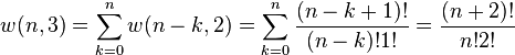
where we have used the following theorem involving binomial coefficients:

Continuing this process, we can see that w(n,g) is just a binomial coefficient

The number of ways that a set of occupation numbers n_i can be realized is the product of the ways that each individual energy level can be populated:

where the approximation assumes that g_i > > 1. Following the same procedure used in deriving the Maxwell–Boltzmann statistics, we wish to find the set of n_i for which W is maximised, subject to the constraint that there be a fixed number of particles, and a fixed energy. The maxima of W and ln(W) occur at the value of N_i and, since it is easier to accomplish mathematically, we will maximise the latter function instead. We constrain our solution using Lagrange multipliers forming the function:

Using the g_i > > 1 approximation and using Stirling's approximation for the factorials gives:

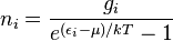
Taking the derivative with respect to n_i, and setting the result to zero and solving for n_i yields the Bose–Einstein population numbers:

It can be shown thermodynamically that β = 1/kT where k is Boltzmann's constant and T is the temperature, and that α = -μ/kT where μ is the chemical potential, so that finally:

Note that the above formula is sometimes written:

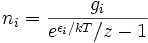
where z = exp(μ / kT) is the absolute activity.

Funny Quotes & Sayings collection's

If women didn't exist, all the money in the world would have no meaning.


I like my whisky old and my women young.


Women are like elephants. Everyone likes to look at them but no-one likes to have to keep one.


Most women are not as young as they are painted.


What a strange thing man is; and what a stranger thing woman.


From 40 feet away she looked like a lot of class. From 15 feet away she looked like something made up to be seen from 40 feet away.


I love women. They're the best thing ever created. If they want to be like men and come down to our level, that's fine.


Women: Can't live with them, can't bury them in the back yard without the neighbors seeing.


To generalize on women is dangerous. To specialize on them is infinitely worse.


Women who seek to be equal with men lack ambition.


One of the most difficult things in the world is to convince a woman that even a bargain costs money.


What would men be without women? Scarce, sir, mighty scarce.


A woman's mind is cleaner than a man's - That's because she changes it more often.


No man knows more about women than I do, and I know nothing.


I'd much rather be a woman than a man. Women can cry, they can wear cute clothes, and they are the first to be rescued off of sinking ships.


When a woman behaves like a man, why doesn't she behave like a nice man ?


Despite my thirty years of research into the woman soul, I have not yet been able to answer the great question that has never been answered: What does a woman want?


Some women hold up dresses that are so ugly and they always say the same thing: 'This looks much better on.' On what? On fire?


Women should have labels on their foreheads saying, 'Government Health Warning: women can seriously damage your brains, current account, confidence, and good standing among your friends'.


The man's desire is for the woman; but the woman's desire is rarely other than for the desire of the man


What is better than wisdom? Woman. And what is better than a good woman? Nothing.


A woman knows how to keep quiet when she is in the right, whereas a man, when he is in the right, will keep on talking.


Woman is a miracle of divine contradictions.


Women are like cars: we all want a Ferrari, sometimes want a pickup truck, and end up with a station wagon.


A woman is like a tea bag. She only knows her strength when put in hot water.


Women are an alien race set down among us.


Women... can't live with 'em... can't shoot 'em.


Being a woman is a terribly difficult task, since it consists principally in dealing with men.


Whatever women do they must do twice as well as men to be thought half as good? Luckily, this is not difficult.


When women go wrong, men go right after them.


If a woman insists on being called Ms, ask her if it stands for miserable.


A woman is an occasional pleasure but a cigar is always a smoke.


There's two theories to arguing with a woman. Neither one works.


The great and almost only comfort about being a woman is that one can always pretend to be more stupid than one is and no one is surprised.


Every time a woman leaves off something she looks better, but every time a man leaves off something he looks worse.


I wonder why it is, that young men are always cautioned against bad girls. Anyone can handle a bad girl. It's the good girls men should be warned against.


Guys are like dogs. They keep coming back. Ladies are like cats. Yell at a cat one time...they're gone.


As long as a woman can look ten years younger than her own daughter, she is perfectly satisfied.


Show me a woman who doesn't feel guilt and I'll show you a man.


I hate housework. You make the beds, you wash the dishes and six months later you have to start all over again.


When women kiss it always reminds me of prize fighter shaking hands.


One should never trust a woman who tells her real age. If she tells that, she'll tell anything.

Life cycle of a star

Fermi-Dirac distribution law & its Derivation

In statistical mechanics, Fermi-Dirac statistics is a particular case of particle statistics developed by Enrico Fermi and Paul Dirac that determines the statistical distribution of fermions over the energy states for a system in thermal equilibrium. In other words, it is a probability of a given energy level to be occupied by a fermion. Fermions are particles which are indistinguishable and obey the Pauli exclusion principle, i.e., no more than one particle may occupy the same quantum state at the same time. Statistical thermodynamics is used to describe the behaviour of large numbers of particles. A collection of non-interacting fermions is called a Fermi gas.

F-D statistics was introduced in 1926 by Enrico Fermi and Paul Dirac and applied in 1926 by Ralph Fowler to describe the collapse of a star to a white dwarf and in 1927 by Arnold Sommerfeld to electrons in metals.

For F-D statistics, the expected number of particles in states with energy ε_i is

where:

is the number of particles in state i,

is the energy of state i,

is the degeneracy of state i (the number of states with energy ),

is the chemical potential (Sometimes the Fermi energy is used instead, as a low-temperature approximation),

is Boltzmann's constant, and

is absolute temperature.

In the case where μ is the Fermi energy and , the function is called the Fermi function:

Fermi-Dirac distribution as a function of temperature. More states are occupied at higher temperatures.

Contents 1. Which distribution to use 2 .A derivation 3. Another derivation 4 .See also

Which distribution to use

Fermi–Dirac and Bose–Einstein statistics apply when quantum effects have to be taken into account and the particles are considered "indistinguishable". The quantum effects appear if the concentration of particles (N/V) ≥ n_q (where n_q is the quantum concentration). The quantum concentration is when the interparticle distance is equal to the thermal de Broglie wavelength i.e. when the wavefunctions of the particles are touching but not overlapping. As the quantum concentration depends on temperature; high temperatures will put most systems in the classical limit unless they have a very high density e.g. a White dwarf. Fermi–Dirac statistics apply to fermions (particles that obey the Pauli exclusion principle), Bose–Einstein statistics apply to bosons. Both Fermi–Dirac and Bose–Einstein become Maxwell–Boltzmann statistics at high temperatures or low concentrations.

Maxwell–Boltzmann statistics are often described as the statistics of "distinguishable" classical particles. In other words the configuration of particle A in state 1 and particle B in state 2 is different from the case where particle B is in state 1 and particle A is in state 2. When this idea is carried out fully, it yields the proper (Boltzmann) distribution of particles in the energy states, but yields non-physical results for the entropy, as embodied in Gibbs paradox. These problems disappear when it is realized that all particles are in fact indistinguishable. Both of these distributions approach the Maxwell–Boltzmann distribution in the limit of high temperature and low density, without the need for any ad hoc assumptions. Maxwell–Boltzmann statistics are particularly useful for studying gases. Fermi–Dirac statistics are most often used for the study of electrons in solids. As such, they form the basis of semiconductor device theory and electronics.

A derivation

Fermi-Dirac distribution as a function of ε. High energy states are less probable. Or, low energy states are more probable.

Consider a single-particle state of a multiparticle system, whose energy is . For example, if our system is some quantum gas in a box, then a state might be a particular single-particle wave function. Recall that, for a grand canonical ensemble in general, the grand partition function is

where

E(s) is the energy of a state s,

N(s) is the number of particles possessed by the system when in the state s,

μ denotes the chemical potential, and

s is an index that runs through all possible microstates of the system.

In the present context, we take our system to be a fixed single-particle state (not a particle). So our system has energy when the state is occupied by n particles, and 0 if it is unoccupied. Consider the balance of single-particle states to be the reservoir. Since the system and the reservoir occupy the same physical space, there is clearly exchange of particles between the two (indeed, this is the very phenomenon we are investigating). This is why we use the grand partition function, which, via chemical potential, takes into consideration the flow of particles between a system and its thermal reservoir.

For fermions, a state can only be either occupied by a single particle or unoccupied. Therefore our system has multiplicity two: occupied by one particle, or unoccupied, called s₁ and s₂ respectively. We see that , , and , . The partition function is therefore

.

For a grand canonical ensemble, probability of a system being in the microstate s_α is given by

.

Our state being occupied by a particle means the system is in microstate s₁, whose probability is

.

is called the Fermi-Dirac distribution. For a fixed temperature T, is the probability that a state with energy ε will be occupied by a fermion. Notice is a decreasing function in ε. This is consistent with our expectation that higher energy states are less likely to be occupied.

Note that if the energy level ε has degeneracy , then we would make the simple modification:

.

This number is then the expected number of particles in the totality of the states with energy ε.

For all temperature T, , that is, the states whose energy is μ will always have equal probability of being occupied or unoccupied.

In the limit , becomes a step function (see graph above). All states whose energy is below the chemical potential will be occupied with probability 1 and those states with energy above μ will be unoccupied. The chemical potential at zero temperature is called Fermi energy, denoted by E_F, i.e.

.

It may be of interest here to note that, in general the chemical potential is temperature-dependent. However, for systems well below the Fermi temperature , it is often sufficient to use the approximation ≈ .

Another derivation

In the previous derivation, we have made use of the grand partition function (or Gibbs sum over states). Equivalently, the same result can be achieved by directly analysing the multiplicities of the system.

Suppose there are two fermions placed in a system with four energy levels. There are six possible arrangements of such a system, which are shown in the diagram below.

   ε1   ε2   ε3   ε4
A  *    *
B  *         *
C  *              *
D       *    *
E       *         *
F            *    *

Each of these arrangements is called a microstate of the system. Assume that, at thermal equilibrium, each of these microstates will be equally likely, subject to the constraints that there be a fixed total energy and a fixed number of particles.

Depending on the values of the energy for each state, it may be that total energy for some of these six combinations is the same as others. Indeed, if we assume that the energies are multiples of some fixed value ε, the energies of each of the microstates become:

A: 3ε

B: 4ε

C: 5ε

D: 5ε

E: 6ε

F: 7ε

So if we know that the system has an energy of 5ε, we can conclude that it will be equally likely that it is in state C or state D. Note that if the particles were distinguishable (the classical case), there would be twelve microstates altogether, rather than six.

Now suppose we have a number of energy levels, labelled by index i , each level having energy ε_i and containing a total of n_i particles. Suppose each level contains g_i distinct sublevels, all of which have the same energy, and which are distinguishable. For example, two particles may have different momenta, in which case they are distinguishable from each other, yet they can still have the same energy. The value of g_i associated with level i is called the "degeneracy" of that energy level. The Pauli exclusion principle states that only one fermion can occupy any such sublevel.

Let w(n, g) be the number of ways of distributing n particles among the g sublevels of an energy level. Its clear that there are g ways of putting one particle into a level with g sublevels, so that w(1, g) = g which we will write as:

We can distribute 2 particles in g sublevels by putting one in the first sublevel and then distributing the remaining n − 1 particles in the remaining g − 1 sublevels, or we could put one in the second sublevel and then distribute the remaining n − 1 particles in the remaining g − 2 sublevels, etc. so that w'(2, g) = w(1, g − 1) + w(1,g − 2) + ... + w(1, 1) or

where we have used the following theorem involving binomial coefficients:

Continuing this process, we can see that w(n, g) is just a binomial coefficient

The number of ways that a set of occupation numbers n_i can be realized is the product of the ways that each individual energy level can be populated:

Following the same procedure used in deriving the Maxwell-Boltzmann distribution, we wish to find the set of n_i for which W is maximised, subject to the constraint that there be a fixed number of particles, and a fixed energy. We constrain our solution using Lagrange multipliers forming the function:

Again, using Stirling's approximation for the factorials and taking the derivative with respect to n_i, and setting the result to zero and solving for n_i yields the Fermi-Dirac population numbers:

It can be shown thermodynamically that β = 1/kT where k is Boltzmann's constant and T is the temperature, and that α = -μ/kT where μ is the chemical potential, so that finally:

Note that the above formula is sometimes written:

where z = exp(μ / kT) is the absolute activity.